The June 2011 issue of The R Journal contains an article on the R package digitize (link to pdf) by Timothée Poisot. This might prove to be a handy tool if you occasionally find yourself needing to retrieve data points from figures in old articles for which you don’t have the raw data. There are a number of other stand-alone software tools to accomplish this same task, such as PlotDigitizer, DataThief, or TechDig (good luck finding that last one). These other programs all work, but I use them so rarely that I typically forget the name of the program and spend more time looking for a new program than it takes to actually digitize the graph. As a result, having a package in R to do the same task might save some exasperation in the future. For an alternative method using ImageJ, see this post.

To get ahold of digitize, simply open up an R session and type the following at the command prompt:
install.packages('digitize') #download the digitize package
library(digitize) #load the digitize package into the workspace

The normal usage routine involves three steps:

cal = ReadAndCal('imagefilename.jpg')

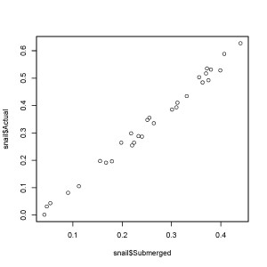
This opens the jpeg in a plotting window and lets you define points on the x and y axes. You must start by clicking on the left-most x-axis point, then the right-most axis point, followed by the lower y-axis point and finally the upper y-axis point. You don’t need to choose the end points of the axis, only two points on the axis that you know the x or y value for. As you click on each of the 4 points, the coordinates are saved in the object cal.

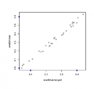
The next step is:
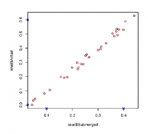
data.points = DigitData(col = 'red')

You return to the figure window, and now you can click on each of the data points you’re interested in retrieving values for. The function will place a dot (colored red in this case) over each point you click on, and the raw x,y coordinates of that point will be saved to the data.points list. When you’re finished clicking points, you need to hit stop or right-click to stop the data point collection.

 

Finally, you need to convert those raw x,y coordinates into the same scale as the original graph. You do this by calling the Calibrate function and feeding it your data.point list, the cal list that contains your 4 control points from the first step, and then 4 numeric values that represent the 4 original points you clicked on the x and y axes. These values should be in the original scale of the figure (i.e. read the values off the graph’s tick marks).

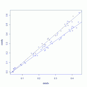
df = Calibrate(data.points, cal, 0.1, 0.4, 0.0, 0.6)
head(df)
x y
1 0.04327273 5.551115e-17
2 0.04763636 3.344262e-02
3 0.05418182 4.327869e-02
4 0.09018182 7.868852e-02
5 0.11200000 1.042623e-01
6 0.15454545 1.967213e-01

The resulting data frame df contains 2 columns, x and y, that contain the scaled values for each point you clicked on the original graph. Note that points that are close to zero aren’t ever going to read exactly zero, but instead will be some very small number in scientific notation (i.e. 5.551115e-17).

There is one major caveat with the use of digitize, that being that your jpeg figure must be rotated correctly so that the x axis is perfectly horizontal and the y-axis is vertical. The digitize package doesn’t make any attempt to correct for rotated axes, and if you input a poorly scanned image that isn’t straight, you’ll get bogus numbers in return. For example, I tried digitizing a rotated version of the above figure (shown below).

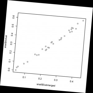
The results I got from digitize on this rotated image do not match the results from the original straight image because my control points on the rotated image are different distances from each other due to the rotation. The plot of the two resulting data sets (straight image in black, rotated image in blue) shows the very different results obtained from an off-kilter image.

Just be careful when creating your input image. If you scan the image slightly off-kilter, open it in an image manipulation program and rotate the figure until the axes are perfectly horizontal/vertical, and then run it through the digitize workflow.

One other minor limitation of digitize is that it only supports jpeg images, so you’ll need to convert tiff, png, or pdf images to jpegs before use.

Edit, October 2011: You might also find this web-based plot digitizer developed by Ankit Rohatgi to be useful: http://arohatgi.info/WebPlotDigitizer/ This program runs inside of your Firefox or Chrome web-browser. Simply drag your plot image onto the application webpage and begin digitizing points. There are helpful tutorials provided as well.