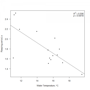
I was fooling around with including a p-value and R2 value on a plot I was putting together, and found myself quickly descending into the world of R graphics esoterica. I wanted to be able to include the values on the fly using values extracted from a linear model summary object, and I wanted to use the proper italics and superscripts for the text. The desired output is shown below. What follows is how I finally generated the plot.

I’ll start with the raw data, fitting the model, and producing the basic plot. The data are in a data frame called ‘test’ that contains two columns of data.
    WTMP     Rasp
1  15.41 1.508667
2  11.03 1.618000
3  15.56 1.616667
4  11.80 2.195333
5  15.70 1.582667
6  19.57 1.286667
7  17.18 1.522667
8  15.36 1.776000
9  15.96 1.664667
10 16.50 1.678000
11 16.78 1.796667
12 16.20 2.016000
13 13.96 2.152000
14 11.32 2.521333
15 11.13 2.484000
I fit the model as follows:
Making the basic plot is straightforward:
plot(test$WTMP, test$Rasp, pch = 20, type = 'p', las = 1,
		xlab = expression(paste('Water Temperature, ',degree,'C',sep ='')),
		ylab = 'Rasping period, s')
And adding the regression line from the linear model is as simple as:
abline(mod1)
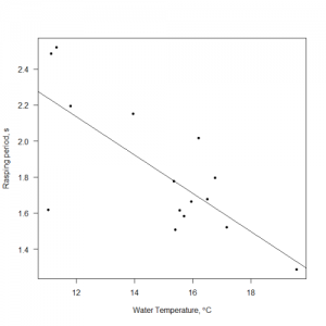
The initial plot looks like this:

That was the simple part. Getting the p-value and R2 onto the plot takes a little more doing. The first step is to extract those values from the model summary object we made. The adjusted R2 value is easily available:
r2 = modsum$adj.r.squared
The p-value for the WTMP variable is buried a little further. The modsum object has a list entry called “coefficients”, which is a 2×4 matrix. The p-value I’m after is in the 2nd row and 4th column. You can see the structure of the coefficients matrix as follows:
modsum$coefficients
which returns:
             Estimate Std. Error   t value     Pr(>|t|)
(Intercept)  3.411080 0.40949496  8.329968 1.432624e-06
WTMP        -0.106269 0.02712375 -3.917932 1.765290e-03
To extract that single p-value in code, I can do the following:
my.p = modsum$coefficients[2,4]
Getting the values stored in r2 and my.p onto the plot takes some head scratching. You could use the text( ) function, or as we’ll see later, the legend( ) function. Those functions are straightforward, but getting nicely formatted text into them requires the use of the bquote( ) function or the expression( ) function and the substitute( ) function. The list of what I want is as follows:
- The R in R2 should be in italics.
- The 2 in R2 should be superscript.
- The numeric R2 value should only be written to 3 significant digits.
- The p of the p-value should be in italics.
- The numeric p-value should only be written to 2 significant digits.
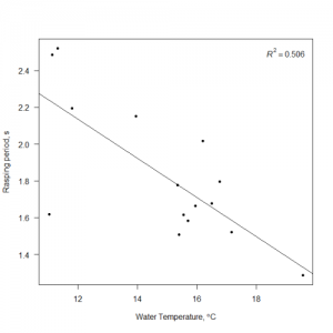
Getting this sort of formatting correct in a R plot can be tricky. I’ll start with the simple case, using text( ) to plot the R2 value.
The code chunk above starts by creating a new object, ‘mylabel‘, that will hold the expression we want to display. On the right side of the equals sign is the bquote( ) function, which creates a ‘call’ object in R. The code inside bquote( ) behaves according to the syntax laid out in plotmath (type ?plotmath in your R terminal to see the help page), except that you can insert other objects inside the .( ) function that will be evaluated like normal R code. Here’s the breakdown of the contents of bquote( ):
- In this case, the bquote starts off with
italic(R), which creates the italicized R. The R is treated as a normal character, not as the name of an object. - The ^ symbol indicates that the next character should be superscript. Thus, the 2 is inserted as a superscript character next to the R. If you wanted a subscript, you would use the square braces instead of ^ (for example:
bquote(italic(R)[italic(adj)]^2== ~.(format(r2,dig = 3)))). If you wanted multiple characters with spaces in the superscript, you’d enclose them in curly braces and quote marks, like so:italic(R)^{'2.12 hi mom'}. - Printing the equals sign inside bquote is accomplished by typing a double equals sign, ==.
- Following the equals sign is the .( ) function, which instructs bquote( ) to evaluate the contents of .( ) like normal R code. In this case, I’ve called the format( ) function.
- Inside the format( ) function, I gave the name of the object holding my numerical R2 value, r2. I also specified that format should print the value out with only 3 significant digits. If you skip this step, R will probably print out many more digits than you wanted.
- If you wanted to include some plain character strings, you can enclose them in quotes if there will be spaces between words, and separate your text from the other parts of the statement using either * (to keep parts together) or ~ (to insert a space between parts). For example:
expression(Adjusted~italic(R)^2 == MYVALUE)will stick the character string “Adjusted” on the front of the output from expression( ), and insert a space between it and the R2 to generate: Adjusted R2=0.506.
The call to text( ) then prints the contents of mylabel on the current figure at the chosen x and y coordinates. You’ll need to specify those coordinates correctly so that everything fits on the plot properly.

You could place lots of labels using the text function, but you do need to be careful about specifying where they end up. While it is possible to insert a newline character (\n) into a text( ) call, getting it to behave as you’d like usually (always?) proves to be an exercise in frustration when trying to print out plotmath expressions (which is what we’re doing when using things like italic( ) and the superscript ^). If you want a second line of text below your first line, you can provide multiple y-values to text( ) along with a vector of expression( ) or bquote( ) output, or use a second text( ) command with a new y-value (in the coordinates of your plot) that will end up below your first text( ) call. Using the legend( ) function is slightly simpler in some respects, because you can feed it locations like ‘topleft‘ or ‘bottomright‘ and legend( ) will try to fit your text in automatically. The legend( ) command will also insert line breaks automatically between elements of a vector of character strings or expressions. You can send a single label like mylabel to legend( ) quite easily. However, passing complicated plotmath-style labels to legend( ) is trickier if you have more than one label you’d like to insert, since legend( ) expects to receive a vector of character strings or expressions. The next section demonstrates how to create a vector of expressions to pass to legend( ).
rp = vector('expression',2)
rp[1] = substitute(expression(italic(R)^2 == MYVALUE),
		list(MYVALUE = format(r2,dig=3)))[2]
rp[2] = substitute(expression(italic(p) == MYOTHERVALUE),
		list(MYOTHERVALUE = format(my.p, digits = 2)))[2]
The code above starts off by creating an empty ‘expression’ vector called rp, length 2, that will hold my two lines of text.
The second line inserts a value into the 1st position of rp, using a convoluted combination of substitute( ) and expression( ).
- Starting with the substitute( ) function, we supply two arguments to substitute. The first is an expression, the 2nd is a list object.
- The expression( ) function is the first argument to substitute( ). This behaves similarly to the bquote( ) function above, in that it takes plotmath-style arguments like italics( ) and ^ for superscript.
- Inside expression( ) you find the
italic(R)^2 ==syntax that we saw above. What’s changed is that there is a new object called ‘MYVALUE’ that didn’t previously exist anywhere. Previously we used the .( ) function with bquote to insert code to be evaluated by R, but that doesn’t work with expression( ). Instead, we’re going to substitute the numerical value into MYVALUE. - The expression object is closed, and the 2nd argument to substitute( ) is the list( ). The list will contain the object MYVALUE, and we’ll assign a value to it.
- The value assigned to MYVALUE is created by
format(r2, digits = 3), which outputs a value with 3 significant digits. The substitute function will find the value stored in MYVALUE and insert it into the expression argument where MYVALUE appears. - After closing off the rest of the parentheses, we’re left with the
[2]hanging off the end of the substitute( ) function. This indicates that we want the 2nd value created by substitute, this is the value that gets inserted intorp[1]. Just trust me, you want the 2nd value.
The process for inserting the next label into rp[2] is similar to the process for creating the 1st label. Once both labels have been created and inserted into rp, you now have the vector of expressions that legend( ) can use to build the legend. We’ll add the completed legend like so:
This makes the final plot I was originally looking for. The R2 value and p-value are inserted in the top corner of the plot, automatically justified so they fit nicely inside the boundary of the figure. If my dataset changes in the future, I can re-run the code above to re-fit the linear model, extract the new R2and p-values, and have them plotted on the figure.

Credit goes t0 Peter Ehlers’ solution in this email thread for helping clarify how this stuff works.