Say you’ve got a bunch of survival/mortality data from an experiment. Maybe you exposed batches of snails to various high temperatures for a few hours, and recorded the number alive and dead in each batch at the end. Now you’d like to report the median lethal temperature (or perhaps a lethal dosage if you were injecting stuff into critters). We can do this fairly quickly using R statistical software to perform a logistic regression and back-calculate the LT50.

This assumes that you already have R installed on your computer and you know how to fire it up.

To start with, we need some data.

In this case, I’ve entered my data into Excel in an arrangement suitable for importing into R. This file, which contains only these data on it, should be saved as a comma-separated-value (.csv) file. Other text file styles would work, but we’ll stick with .csv. You’ll need to know the path to the directory where this file is stored so that you can find it with R.

With R open, we’ll load the .csv file into the R workspace by entering the following command at the prompt:

> data = read.csv("D:/directory/data.csv")

where D:/directory/ is the path to our file, and data.csv is the name of the file we created in Excel. The data are now entered into a data frame called 'data'.

We can examine the contents of  'data' by simply typing the name of the data frame at the prompt:

> data

which would return something like this:

   temperature alive dead
1           38    20    0
2           40    20    0
3           40    20    0
4           40    20    0
5           42    19    1
6           42    14    6
7           42    15    5
8           44     5   15
9           44     3   17
10          44     2   18
11          47     0   20
12          47     0   20
13          47     0   20

That looks about right. There are data from the 13 different trials I ran, with the temperature, number alive, and number dead given for each trial. Having the numbers as alive + dead is necessary here, so if you recorded your data as % survival or % mortality, convert the values back into counts.

Now if you’re having trouble importing your data, you could type it directly into a data frame in R as follows:

> data = data.frame(temperature = 
   c(38,40,40,40,42,42,42,44,44,44,47,47,47),
   alive = c(20,20,20,20,19,14,15,5,3,2,0,0,0),
   dead = c(0,0,0,0,1,6,5,15,17,18,20,20,20))

That recreates the data table from above.

Now that your data are in the workspace, let’s attach them so that we can refer to each column by its header directly:

> attach(data)

If you then typed > temperature, R would respond with all the contents of the temperature column.

Next it’s necessary to create a separate array of our response variables (alive and dead):

> y = cbind(alive, dead)

At this point we can run the generalized linear model using a binomial distribution to fit a curve to temperature and alive/dead data:

> model.results = glm(y ~ temperature, binomial)

In that line, we created an object model.results to hold our output, and called the glm function. We supplied glm with our response variable and the treatment levels y ~ temperature, followed by the distribution we want to use binomial . Since our response variable only has two states (alive or dead), the binomial distribution is the weapon of choice.

You can check the results of the models by typing the name of the model object you just created:

> model.results

which outputs the following for our data above:

Call: glm(formula = y ~ temperature, family = binomial)

Coefficients:
(Intercept) temperature 
     69.113      -1.609

Degrees of Freedom: 12 Total (i.e. Null); 11 Residual
Null Deviance:      252.2 
Residual Deviance: 8.309     AIC: 29.29

It’s worth noting that the Residual Deviance here (8.309) is less than our Residual Degrees of Freedom (11), meaning that our data are not overdispersed. If the Residual Deviance was something large like 20 compared to our 11 Residual Degrees of freedom, it might be worth trying a log-transformation on the treatment values. This might be the case if you were administering dosages of some drug over a very wide range of concentrations. To carry out a logistic regression on our log-transformed data, we’d simply modify the glm call slightly:

> model.results = glm(y ~ log(temperature), binomial)

which calculates the natural log of each treatment level prior to carrying out the regression.

You can also print out the model results in summary format, which will also show you standard error estimates, z-values, and P-values for the estimates of the intercept and slope coefficients of the logistic regression:

> summary(model.results)

The summary results look like this:

Call:
glm(formula = y ~ temperature, family = binomial)

Deviance Residuals: 
     Min       1Q   Median      3Q     Max 
-1.30305 -0.24134 -0.05082 0.59144 1.74125

Coefficients:
           Estimate Std. Error z value Pr(>|z|) 
(Intercept) 69.1126     9.0186   7.663 1.81e-14 ***
temperature -1.6094     0.2103  -7.653 1.96e-14 ***
---
Signif. codes: 0 '***' 0.001 '**' 0.01 '*' 0.05 '.' 0.1 ' ' 1

(Dispersion parameter for binomial family taken to be 1)

Null deviance: 252.1776 on 12 degrees of freedom
Residual deviance: 8.3088 on 11 degrees of freedom
AIC: 29.294
Number of Fisher Scoring iterations: 5

To calculate what the median lethal temperature in the experiment was, we’ll use a function in the MASS library that comes with the base installation of R. Load the MASS library:

> library(MASS)

 The MASS library has a handy function called dose.p that will calculate any fractional dosage value you want (i.e. LT50, LT90, LT95 etc). Call dose.p as follows:

> dose.p(model.results, p = 0.5)

Note that we input our model.results object as the input, and then input our desired level (p=0.5, which is 50% survival).
The results from dose.p will look like this:

             Dose        SE
p = 0.5: 42.94194 0.1497318

In this case, the value given under Dose is the median lethal dose (i.e. temperature), 42.94194 (we’ll drop a few significant digits and call it 43°C when it’s time to write things up). Note here that if you had to log transform your data during the glm call above, the value returned in Dose will also be log-transformed (3.7598 if we did this to the data above). You would convert it back to natural units using the exponential command: > exp(3.7598) which would return ~42.9°C if we used this data set.

If we also wanted to know what dosage gave 90% survival, we’d call dose.p as such:

> dose.p(model.results, p = c(0.5, 0.9))

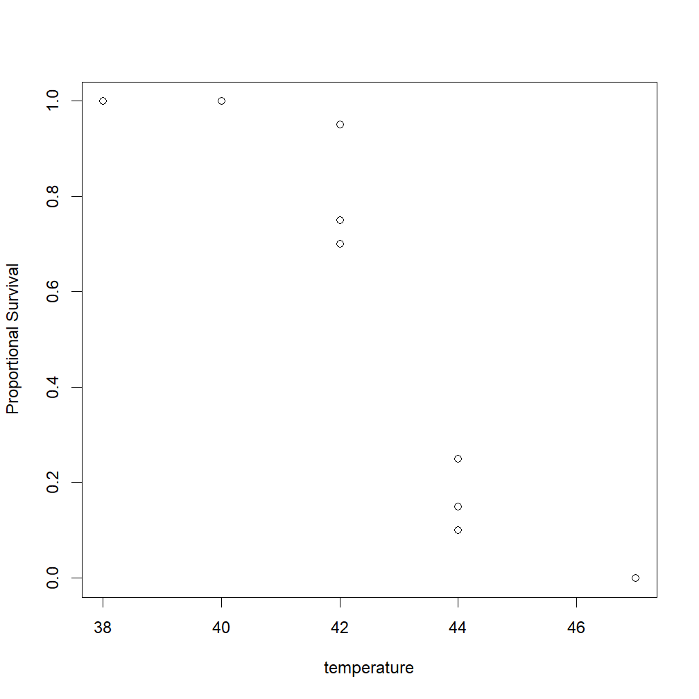
It might also be useful to have a graph of % Survival and a logistic curve fit to the data for making a figure. Let’s do that.

To begin, we can plot our original alive/dead data as % survival by just dividing the number alive by the total number of animals per trial when we call the plot command:

> plot(temperature, (alive / (alive + dead)), ylab = "Proportional Survival")

Note the (alive / (alive + dead)) section in there. That tells R that we want our y-values to be the number alive divided by the total number of animals per trial (a proportion between 0 and 1).
The resulting plot looks like this:

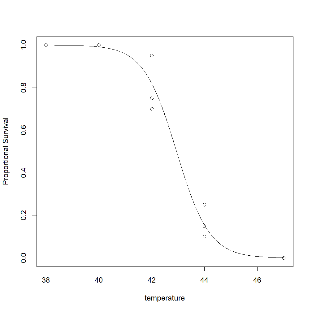
Next we need to come up with a way to plot a logistic curve over our raw data values. To do this, we’ll have to define a function that will calculate y-values along a logistic curve. We do this as follows:

> logisticline = function(z) {
	eta = 69.1126 + -1.6094 * z;
	1 / (1 + exp(-eta))
	}

In the 2nd line of that equation, we write a little formula for ‘eta’ using the values 69.1126 and -1.6094, which were the intercept and slope that were reported in our summary(model.results) given above. Substitute your own slope and intercept in there, but leave the ‘z’ alone. The third line is the standard logistic function used to calculate the value ‘logisticline’ for each input value z. Leave the third line alone.

Now we need to create a vector of temperature values that will be used as input to our function ‘logisticline’ to create the y-values to plot our curve.

> x = seq(38, 47, 0.01)

In that line, we define an object ‘x’ and fill it with a sequence (i.e. ‘seq’) of numbers from 38 to 47 (my temperature limits) using a step size of 0.01. The small step size ensures that the curve will look smooth. If you don’t specify a step size, the ‘seq’ command will step by 1, making for a non-curvy curve in this case.

Finally, we can add this line to our existing plot. Note that we’ll call the ‘logisticline’ function we just defined, and supply it with the vector ‘x’, so that the y-values plotted on the graph are calculated by plugging each value of x into the logistic equation and plotting the resulting proportional survival:

> lines(x, logisticline(x), new = TRUE)

The resulting output should look something like this:

Should you want to make your own plots look more presentable, there are some tips for modifying the output of the plot in this post.